4. Data Structures of the NumPy Library
NumPy Library
The NumPy library includes tools for numerical computing, the most important of which is ndarray (or array), i.e., an array that can represent vectors, matrices, and any multi-dimensional arrays. NumPy arrays enable numerical computing in different ways than regular lists (ndarray = n-dimensional array). NumPy is optimized for mathematical operations, meaning that their computation is significantly faster than using list data structures, for example.
NumPy contains numerous functions for array manipulation, matrix computation, and statistical calculation. The implementations of NumPy arrays and functions are highly optimized for speed.
Importing the NumPy Library
The numpy library is used in the code with the import numpy command. The established practice is to use the alias np:
import numpy as np
After this, NumPy functions can be called in the code using the abbreviation np.
NumPy Array (array)
Arrays can be created from Python lists (or tuples) using the numpy.array function.
import numpy as np


# Creating a one-dimensional array with four elements (i.e., a vector)


vector = np.array([10, 20, 30, 40])
vector2 = np.array([1,3,6,9])


print("Vector: ", vector)
print("Vector2: ", vector2)
Vector:  [10 20 30 40]
Vector2:  [1 3 6 9]
Referring to array elements works like with lists:
first = vector[0] # 10
print("First: ", first)
second = vector[1] # 20
print("Second: ", second)
last_1 = vector[3] # 40
print("Last1: ", last_1)
last_2 = vector[-1] # 40, the last element
print("Last2: ", last_2)
last_2 = vector[-2] # 30, the second to last element
print("Last2: ", last_2)
First:  10
Second:  20
Last1:  40
Last2:  40
Last2:  30
Unlike lists, NumPy arrays cannot contain elements of different types. If the list used for creation contains elements of different types, NumPy will convert all elements to the "most general" data type.
list1 = [1, 3, 3.1]
nparray1 = np.array(list1)
print(nparray1)  # all floats


list2 = [1, 2.1, "3"]
nparray2 = np.array(list2)
print(nparray2)  # all strings
[1.  3.  3.1]
['1' '2.1' '3']


A two-dimensional NumPy array, or matrix, can be created in the same way from a list of lists:


```python
matrix = np.array([[10, 20, 30],
                   [40, 50, 60]])


print(matrix)
[[10 20 30]
 [40 50 60]]
Elements in two-dimensional NumPy arrays can be accessed with the array[row, column] notation.
The familiar notation from regular lists array[row][column] also works, but it is more cumbersome.
first_first = matrix[0, 0] # 10
second_second = matrix[1, 1] # 50
second_last = matrix[1, -1] # 60
second_last2 = matrix[1][-1] # 60


print(second_last)
print(second_last2)
60
60
Similarly, a matrix can also be multi-dimensional, for example, 3-dimensional.
The dimensions of an array can be determined with the numpy.ndim() function.
The numpy.shape() function returns the dimensions of the array's extents.
The dimension (number of elements) of an individual extent can be obtained with the len() function.
print(np.ndim(matrix))
print(np.shape(matrix))
print(len(matrix[1]))
2
(2, 3)
3
An array can also be created with NumPy's built-in initialization functions:
numpy.zeros()creates an array where all elements are zerosnumpy.arange()works like the range function used with for-loopsnumpy.linspace()fills the array with evenly spaced floating-point numbers
# Vector
print(np.zeros(10))
# Matrix
print(np.zeros([5, 3])) # would also work with a tuple np.zeros((5, 3))


print("\n")


print(np.arange(1, 11)) # start, end. End is not included
print(np.arange(0, 101, 10)) # start, end, step
print(np.arange(10, 0, -1)) # start, end, step


print("\n")


print(np.linspace(0, 10, 5)) # start, end, number of numbers
[0. 0. 0. 0. 0. 0. 0. 0. 0. 0.]
[[0. 0. 0.]
 [0. 0. 0.]
 [0. 0. 0.]
 [0. 0. 0.]
 [0. 0. 0.]]


[ 1  2  3  4  5  6  7  8  9 10]
[  0  10  20  30  40  50  60  70  80  90 100]
[10  9  8  7  6  5  4  3  2  1]


[ 0.   2.5  5.   7.5 10. ]
Sometimes it may be necessary to change the shape of a matrix, which can be done with the reshape() function:
```python
taul1 = np.arange(0,24,2)
print(taul1)


print("\n")


taul2 = taul1.reshape((3, 4))
print(taul2)


print("\n")


taul3 = taul1.reshape((6, 2))
print(taul3)
[ 0  2  4  6  8 10 12 14 16 18 20 22]


[[ 0  2  4  6]
 [ 8 10 12 14]
 [16 18 20 22]]


[[ 0  2]
 [ 4  6]
 [ 8 10]
 [12 14]
 [16 18]
 [20 22]]
Slicing NumPy Arrays
Slicing NumPy arrays works in the same way as slicing lists. In the notation [start:stop:step], the stop element is thus not included in the slice anymore. The step part is not mandatory.
vector = np.arange(10, 110, 10)
print(vector)


print("\n")


slice1 = vector[2:5]
print(slice1)


print("\n")


print(vector[-2:3:-1])


print("\n")


matrix = np.array([[1, 2, 3, 4],
                   [5, 6, 7, 8],
                   [9, 10, 11, 12]])
print(matrix)


print("\n")


print(matrix[1, 1:3])


print("\n")


print(matrix[2, -2:])
[ 10  20  30  40  50  60  70  80  90 100]


[30 40 50]


[90 80 70 60 50]


[[ 1  2  3  4]
 [ 5  6  7  8]
 [ 9 10 11 12]]


[6 7]


[11 12]
NumPy also offers a convenient : indexing. The : index means all indices of that dimension:
M = np.array([[1, 2, 3, 4],
              [5, 6, 7, 8],
              [9, 10, 11, 12]])


# The third column of all rows of matrix M
print(M[:, 2]) # array([ 3,  7, 11])
# All columns of the second row of matrix M
print(M[1, :]) # array([5, 6, 7, 8])
# This is also equivalent to the abbreviated notation, where the columns can be omitted
print(M[1])    # array([5, 6, 7, 8])
[ 3  7 11]
[5 6 7 8]
[5 6 7 8]
Slicing NumPy arrays is thus implemented with much simpler syntax than python lists:
# extracting "1st column" from a "2D" python list
x = [["a", "b"], ["c", "d"]]
print([x[0][0], x[1][0]])


# the same with a NumPy array
np_x = np.array(x)
print(np_x[:,0])
['a', 'c']
['a' 'c']
Slicing does not, however, create a new array but rather a kind of "view" to the original array (this is related to optimization of memory handling). Therefore, changes made to the view also affect the original array:
arr1 = np.array([1, 2, 3, 4, 5, 6, 7, 8])
arr2 = arr1[2:5]


print(arr2)  # [3 4 5]


arr2[1] = 10


print(arr2) # [ 3 10  5]
print(arr1)  # arr1 has also changed! [ 1  2  3 10  5  6  7  8]


# a new array can be obtained with the copy() function


arr3 = arr1[5:8].copy()
arr3[1] = 100


print(arr3)
print(arr1)  # has not changed
[3 4 5]
[ 3 10  5]
[ 1  2  3 10  5  6  7  8]
[  6 100   8]
[ 1  2  3 10  5  6  7  8]
Operations with NumPy arrays
A NumPy array can be multiplied/divided/added, etc., with a scalar value (number), in which case NumPy performs the operation on each element separately:
vector = np.array([1, 3, 7, 9, 11])
v2 = vector + 5
print(v2)


print("\n")


v3 = (vector ** 2)/2
print(v3)
[ 6  8 12 14 16]

[ 0.5  4.5 24.5 40.5 60.5]
NumPy arrays can also be added, multiplied, and divided with each other. The operations are done element-wise, so the dimensions of the arrays must match.
vector1 = np.array([1, 3, 7, 9, 11])
vector2 = np.array([0.5 , -1, 1, 0.1, 3])


print(vector1 + vector2)


print("\n")


print(vector1 * vector2)


print("\n")


print((vector1 / vector2)**2)


print("\n")


print(vector1 + np.array([3,4,5])) # error message, dimensions do not match
[ 1.5  2.   8.   9.1 14. ]

[ 0.5 -3.   7.   0.9 33. ]

[4.00000000e+00 9.00000000e+00 4.90000000e+01 8.10000000e+03
 1.34444444e+01]

---------------------------------------------------------------------------

ValueError                                Traceback (most recent call last)

~\AppData\Local\Temp\ipykernel_18192\3897137633.py in <module>
     14 print("\n")
     15
---> 16 print(vector1 + np.array([3,4,5])) # error message, dimensions do not match

ValueError: operands could not be broadcast together with shapes (5,) (3,)
In the following, each row of matrix M is multiplied element-wise by vector a (this is not the dot product of matrices).
M = np.array([[1, 2, 3, 4],
              [5, 6, 7, 8],
              [9, 10, 11, 12]])
a = np.array([1, 2, 3, 4])
print(M * a)
[[ 1  4  9 16]
 [ 5 12 21 32]
 [ 9 20 33 48]]
Using NumPy's own mathematical functions, calculations can be performed element-wise on a NumPy array
import math
vector  = np.arange(0,370,10)
print(np.radians(vector))
print('\n')
print(np.sin(np.radians(vector)))
[0.         0.17453293 0.34906585 0.52359878 0.6981317  0.87266463
 1.04719755 1.22173048 1.3962634  1.57079633 1.74532925 1.91986218
 2.0943951  2.26892803 2.44346095 2.61799388 2.7925268  2.96705973
 3.14159265 3.31612558 3.4906585  3.66519143 3.83972435 4.01425728
 4.1887902  4.36332313 4.53785606 4.71238898 4.88692191 5.06145483
 5.23598776 5.41052068 5.58505361 5.75958653 5.93411946 6.10865238
 6.28318531]


[ 0.00000000e+00  1.73648178e-01  3.42020143e-01  5.00000000e-01
  6.42787610e-01  7.66044443e-01  8.66025404e-01  9.39692621e-01
  9.84807753e-01  1.00000000e+00  9.84807753e-01  9.39692621e-01
  8.66025404e-01  7.66044443e-01  6.42787610e-01  5.00000000e-01
  3.42020143e-01  1.73648178e-01  1.22464680e-16 -1.73648178e-01
 -3.42020143e-01 -5.00000000e-01 -6.42787610e-01 -7.66044443e-01
 -8.66025404e-01 -9.39692621e-01 -9.84807753e-01 -1.00000000e+00
 -9.84807753e-01 -9.39692621e-01 -8.66025404e-01 -7.66044443e-01
 -6.42787610e-01 -5.00000000e-01 -3.42020143e-01 -1.73648178e-01
 -2.44929360e-16]
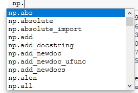
Jupyter notebook also has a simple function for listing available functions: type np. and press the tab key, which will give a list of functions.
NumPy also includes statistical functions for arrays:
numpy.sumcalculates the sum of elementsnumpy.prodcalculates the product of elementsnumpy.meancalculates the mean of elementsnumpy.mediancalculates the median of elementsnumpy.stdcalculates the standard deviation of elementsnumpy.amaxreturns the maximum valuenumpy.aminreturns the minimum value
these can also be called in the style of array.sum()
arr = np.array([1, 56, 5, 10, 11, 2])
print("mean:", np.mean(arr))
print("median:", np.median(arr))
print("largest:", np.max(arr))
print("smallest:", np.amin(arr))
print("sum:", np.sum(arr))
print("sum, another way:", arr.sum())
mean: 14.166666666666666
median: 7.5
largest: 56
smallest: 1
sum: 85
sum, another way: 85
NumPy Array vs. List
Thus, computing with NumPy arrays differs in principle from similar operations on Python lists:
l1 = [1, 2, 3]
l2 = [10, 20, 30]
print(l1+l2)
print(l1*2)


print(15*'-')


np_l1 = np.array(l1)
np_l2 = np.array(l2)
print(np_l1+np_l2)
print(np_l2)
[1, 2, 3, 10, 20, 30]
[1, 2, 3, 1, 2, 3]
---------------
[11 22 33]
[10 20 30]
If you wanted to multiply all elements in a Python list by two, you would need to use a for-loop
l1 = [1, 2, 3]
l2 = []
for i in l1:
  l2.append(i*2)


print(l2)


# list comprehension can also be used:
l3 = {x * 2 for x in l1}
print(l3)
[2, 4, 6]
{2, 4, 6}
Filtering a NumPy Array with a Boolean Array
A NumPy array can be filtered by providing a Boolean array of the same length for "slicing," where each element is either True or False:
arr = np.array([1, 2, 3, 4, 5, 6])
arr2 = np.array([True, False, False, True, True, False])
print(arr[arr2])
[1 4 5]
A True/False array can be easily obtained from a NumPy array, for example, with comparison operators
arr = np.array([1, 2, 3, 4, 5, 6])
arr2 = arr % 2 == 0 # remainder is 0, i.e., an even number
print(arr2)
[False True False True False True]
By combining these two things, we see that a NumPy array can be easily filtered:
arr = np.array([1, 2, 3, 4, 5, 6])
arr3 = arr[arr % 2 == 0]
arr4 = arr[arr > 2]
print(arr3)
print(arr4)
[2 4 6]
[3 4 5 6]
# let's assume that types and readings correspond to each other in order:


types = np.array(['A', 'C', 'B', 'A', 'A', 'D', 'B', 'C'])
readings = np.array([15, 21, 13, 32, 34, 45, 6, 1])


# select readings of type A
print(readings[types == 'A'])


# select readings of types A and B.
# Keywords and or or do not work with Boolean arrays, you must use & or |
print(readings[(types == 'A') | (types == 'B')])
[15 32 34]
[15 13 32 34  6]
Using a Boolean array, you can also change only the filtered values:
arr1 = np.array([1, 2, 3, 4, 5, 6])


# filter even numbers and change them to zeros


arr2 = arr1 % 2 == 0
print(arr2)  # Boolean array


arr1[arr2] = 0   # or directly arr1[arr1 % 2 == 0] = 0


print(arr1)
[False  True False  True False  True]
[1 0 3 0 5 0]
Filtering with a Boolean array gives a copy of the array/part of the array, not a view like slicing:
arr1 = np.array([1, 2, 3, 4, 5, 6])


arr2 =  arr1[arr1 % 2 == 0]
print(arr2)


arr2[0] = 100


print(arr2)
print(arr1)
[2 4 6]
[100   4   6]
[1 2 3 4 5 6]
Sorting
array.sort() sorts the array, numpy.sort(array) gives a sorted copy of the array.
Neither sorting method allows specifying the order as ascending/descending. Often the trick array[::-1] is used to reverse the order of the elements in the array.
arr1 = np.array([3, 5, 1, -2, 0, 4])
print(arr1)


arr1.sort()
print(arr1)


print('\n----------\n')


arr1 = np.array([3, 5, 1, -2, 0, 4])
print(arr1)


arr2 = np.sort(arr1)
print(arr2)
print(arr1)


arr3 = np.sort(arr1)[::-1]
print(arr3)
[ 3  5  1 -2  0  4]
[-2  0  1  3  4  5]


----------


[ 3  5  1 -2  0  4]
[-2  0  1  3  4  5]
[ 3  5  1 -2  0  4]
[ 5  4  3  1  0 -2]