8. Handling DataFrame - Part 2
Combining DataFrames
Often data is spread across several different files and even in different formats, so combining the data into one DataFrame (or Series) may need to be done before starting the analysis.
pandas.merge
The pandas.merge() function combines DataFrames based on a key in a similar way to the join operation in relational databases.
If the function is not told which field to combine on, merge uses overlapping (same) column names as the merge field. However, it is smarter to specify the field used for merging with the on parameter.
import pandas as pd


df1 = pd.DataFrame({'key': ['b', 'b', 'a', 'c', 'a', 'a', 'b'],
                    'data1': range(7)})


df2 = pd.DataFrame({'key': ['a', 'b', 'd'],
                    'data2': range(3)})


print(df1)


print('\n------------------\n')


print(df2)


print('\n------------------\n')


df3 = pd.merge(df1, df2)


# better: df3 = pd.merge(df1, df2, on = 'key')


print(df3)
  key  data1
0     b      0
1     b      1
2     a      2
3     c      3
4     a      4
5     a      5
6     b      6


------------------


  key  data2
0     a      0
1     b      1
2     d      2


------------------


  key  data1  data2
0     b      0      1
1     b      1      1
2     b      6      1
3     a      2      0
4     a      4      0
5     a      5      0
If the names of the columns used for merging differ in the DataFrames, they can be specified separately with the left_on and right_on parameters:
df1 = pd.DataFrame({'key1': ['b', 'b', 'a', 'c', 'a', 'a', 'b'],
                    'data1': range(7)})


df2 = pd.DataFrame({'key2': ['a', 'b', 'd'],
                    'data2': range(3)})


print(df1)


print('\n------------------\n')


print(df2)


print('\n------------------\n')


df3 = pd.merge(df1, df2, left_on = 'key1', right_on = 'key2')


print(df3)
  key1  data1
0      b      0
1      b      1
2      a      2
3      c      3
4      a      4
5      a      5
6      b      6


------------------


  key2  data2
0      a      0
1      b      1
2      d      2


------------------
key1 data1 key2 data2 0 b 0 b 1 1 b 1 b 1 2 b 6 b 1 3 a 2 a 0 4 a 4 a 0 5 a 5 a 0
In the previous examples, keys c and d did not come into the combination at all, because they were not present in both DataFrames. By default, merge performs an "inner"-type join, where the result includes only those keys that are in both DataFrames.
And because df1 had multiple rows with keys a and b, the combination also included multiple of these.
The type of join can be specified with the how parameter, the options are:
innerkeys that are in bothleftkeys that are in the left (first) DataFramerightkeys that are in the right (second) DataFrameouterkeys that are in either of the DataFrames
df1 = pd.DataFrame({'key': ['b', 'b', 'a', 'c', 'a', 'a', 'b'],
                    'data1': range(7)})


df2 = pd.DataFrame({'key': ['a', 'b', 'd'],
                    'data2': range(3)})


print(df1)


print('\n------------------\n')


print(df2)


print('\n------------------\n')


df3 = pd.merge(df1, df2, on = 'key', how = 'outer')


print(df3)
  key  data1
0     b      0
1     b      1
2     a      2
3     c      3
4     a      4
5     a      5
6     b      6


------------------


  key  data2
0     a      0
1     b      1
2     d      2


------------------


  key  data1  data2
0     b    0.0    1.0
1     b    1.0    1.0
2     b    6.0    1.0
3     a    2.0    0.0
4     a    4.0    0.0
5     a    5.0    0.0
6     c    3.0    NaN
7     d    NaN    2.0
If both have several rows with the same key, merge will create all possible "combinations" of these, i.e., if the 1st DataFrame has, for example, 4 rows with key a and the second has 3, the combination will have 4 x 3 = 12 rows with key a.
df1 = pd.DataFrame({'key': ['b', 'b', 'a', 'a', 'a', 'a', 'b'],
                    'data1': range(7)})


df2 = pd.DataFrame({'key': ['a', 'a', 'b'],
                    'data2': range(3)})


print(df1)


print('\n------------------\n')


print(df2)


print('\n------------------\n')


df3 = pd.merge(df1, df2, on = 'key')


print(df3)
key data1 0 b 0 1 b 1 2 a 2 3 a 3 4 a 4 5 a 5 6 b 6
------------------


  key  data2
0     a      0
1     a      1
2     b      2


------------------


   key  data1  data2
0      b      0      2
1      b      1      2
2      b      6      2
3      a      2      0
4      a      2      1
5      a      3      0
6      a      3      1
7      a      4      0
8      a      4      1
9      a      5      0
10     a      5      1
What if the DataFrames to be merged have columns with the same name? pandas adds a suffix (by default _x and _y) to the column names. You can define your own suffixes with the parameter suffixes=('_1','_2').
df1 = pd.DataFrame({'key': ['b', 'b', 'a', 'c', 'a', 'a', 'b'],
                    'data1': range(7)})


df2 = pd.DataFrame({'key': ['a', 'b', 'd'],
                    'data1': range(3)})


print(df1)


print('\n------------------\n')


print(df2)


print('\n------------------\n')


df3 = pd.merge(df1, df2, on = 'key')


print(df3)


print('\n------------------\n')


df4 = pd.merge(df1, df2, on = 'key', suffixes=('_1','_2'))


print(df4)
  key  data1
0     b      0
1     b      1
2     a      2
3     c      3
4     a      4
5     a      5
6     b      6


------------------


  key  data1
0     a      0
1     b      1
2     d      2


------------------


  key  data1_x  data1_y
0     b        0        1
1     b        1        1
2     b        6        1
3     a        2        0
4     a        4        0
5     a        5        0


------------------


  key  data1_1  data1_2
0     b        0        1
1     b        1        1
2     b        6        1
3     a        2        0
4     a        4        0
5     a        5        0
Merging can also be done using multiple fields:
df1 = pd.DataFrame({'key1': ['foo', 'foo', 'bar'],
                    'key2': ['one', 'two', 'one'],
                    'lval': [1, 2, 3]})


df2 =  right = pd.DataFrame({'key1': ['foo', 'foo', 'bar', 'bar'],
                             'key2': ['one', 'one', 'one', 'two'],
                             'rval': [4, 5, 6, 7]})


print(df1)


print('\n-------------\n')


print(df2)


print('\n-------------\n')


pd.merge(df1, df2, on=['key1', 'key2'], how='outer')
  key1 key2  lval
0  foo  one     1
1  foo  two     2
2  bar  one     3


-------------


  key1 key2  rval
0  foo  one     4
1  foo  one     5
2  bar  one     6
3  bar  two     7


-------------
| key1 | key2 | lval | rval | |
|---|---|---|---|---|
| 0 | foo | one | 1.0 | 4.0 |
| 1 | foo | one | 1.0 | 5.0 |
| 2 | foo | two | 2.0 | NaN |
| 3 | bar | one | 3.0 | 6.0 |
| 4 | bar | two | NaN | 7.0 |
Merging is often done based on the index (row header) instead of a data field. For this, there is the parameter left_index=True, which indicates that in the first DataFrame, the merging field is the index. Similarly, right_index=True.
join
Merging based on the index can also be done with the DataFrame's join method. It defaults to a left-type merge, but the how parameter can be used to specify the type (left, right, outer, inner).
If there are columns with the same name in the DataFrame, join will not succeed without the lsuffix and/or rsuffix parameters.
The join method can also be used to merge several DataFrames at once
df.join([df1, df2, df3])
import pandas as pd
technologies = {
    'Courses':["Python","R","Matlab","C++"],
    'Credits' :[4,5,3,6],
    'Duration':['40days','50days','30days','60days'],
              }
index_labels=['r1','r2','r3','r4']
df1 = pd.DataFrame(technologies,index=index_labels)


print("DF1\n",df1)


technologies2 = {
    'Courses':["Python","Java","Python","Go"],
    'Price':[2000,2500,1200,3000]
              }
index_labels2=['r1','r6','r3','r5']
df2 = pd.DataFrame(technologies2,index=index_labels2)


print("\nDF2\n",df2)
DF1 Courses Credits Duration r1 Python 4 40 days r2 R 5 50 days r3 Matlab 3 30 days r4 C++ 6 60 days
DF2
    Courses  Price
r1  Python   2000
r6    Java   2500
r3  Python   1200
r5      Go   3000
# pandas join
df3=df1.join(df2, lsuffix="_left", rsuffix="_right")
print(df3)
   Courses_left  Credits Duration Courses_right   Price
r1       Python        4   40 days        Python  2000.0
r2            R        5   50 days           NaN     NaN
r3       Matlab        3   30 days        Python  1200.0
r4          C++        6   60 days           NaN     NaN
# pandas Inner join DataFrames
df3=df1.join(df2, lsuffix="_left", rsuffix="_right", how='inner')
print(df3)


# Outputs
#   Courses_left    Fee Duration Courses_right  Discount
#r1        Spark  20000   30 days         Spark      2000
#r3       Python  22000   35 days        Python      1200
   Courses_left  Credits Duration Courses_right  Price
r1       Python        4   40 days        Python   2000
r3       Matlab        3   30 days        Python   1200
pandas.concat
DataFrames (and Series) can also be combined ("chained") using the concat function. By default, concat chains the rows, but with the parameter axis=1, the columns are chained.
The keys parameter can be used to define titles for the original rows/columns, thus obtaining a multi-level index for either rows or columns.
import numpy as np
df1 = pd.DataFrame(np.arange(6).reshape(3, 2), index=['a', 'b', 'c'], columns=['one', 'two'])
df2 = pd.DataFrame(5 + np.arange(4).reshape(2, 2), index=['a', 'd'], columns=['three', 'two'])


print('\n-------DF1---------\n')
print(df1)


print('\n-------DF2---------\n')


print(df2)


print('\n------------------\n')


print(pd.concat([df1, df2]))


print('\n------------------\n')


print(pd.concat([df1, df2], axis=1))
-------DF1---------


   one  two
a    0    1
b    2    3
c    4    5


-------DF2---------


   three  two
a      5    6
d      7    8


------------------


   one  two  three
a  0.0    1    NaN
b  2.0    3    NaN
c  4.0    5    NaN
a  NaN    6    5.0
d  NaN    8    7.0


------------------


   one  two  three  two
a  0.0  1.0    5.0  6.0
b  2.0  3.0    NaN  NaN
c  4.0  5.0    NaN  NaN
d  NaN  NaN    7.0  8.0
combine_first
The combine_first method of a DataFrame can be used to "fill in the gaps", meaning that NaN values in a DataFrame are replaced with values found in another DataFrame.
df1 = pd.DataFrame({'a':[4,6,7,np.nan, 5], 'b':[5, np.nan, 87,2,np.nan]})
df2 = pd.DataFrame({'a':[1,np.nan,2,6, 5, 5], 'b':[5, 1, 45,2,7, 8], 'c':[5, np.nan, 87,2,0, 9]})


print('\n-------DF1---------\n')
print(df1)


print('\n-------DF2---------\n')


print(df2)


print('\n------------------\n')


print(df1.combine_first(df2))
-------DF1---------


     a     b
0  4.0   5.0
1  6.0   NaN
2  7.0  87.0
3  NaN   2.0
4  5.0   NaN


-------DF2---------


     a   b     c
0  1.0   5   5.0
1  NaN   1   NaN
2  2.0  45  87.0
3  6.0   2   2.0
4  5.0   7   0.0
5  5.0   8   9.0


------------------


     a     b     c
0  4.0   5.0   5.0
1  6.0   1.0   NaN
2  7.0  87.0  87.0
3  6.0   2.0   2.0
4  5.0   7.0   0.0
5  5.0   8.0   9.0
Data compilation
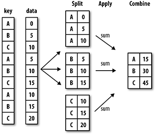
groupby
The groupby method can be used to group data according to a given field. The principle is referred to as split-apply-combine, which means first dividing the data into groups, then performing some operation on the groups, and finally combining the results:
In the Titanic example, the number of survivors was calculated by passenger class (Pclass):
df = pd.read_csv('Datasets/titanic.csv', index_col=0)


df
<style>
    .dataframe thead th {
        text-align: right;
    }
</style>
<table border="1" class="dataframe">
  <thead>
    <tr style="text-align: right;">
      <th></th>
      <th>Survived</th>
      <th>Pclass</th>
      <th>Name</th>
      <th>Sex</th>
      <th>Age</th>
      <th>SibSp</th>
      <th>Parch</th>
      <th>Ticket</th>
      <th>Fare</th>
      <th>Cabin</th>
      <th>Embarked</th>
    </tr>
    <tr>
      <th>PassengerId</th>
      <th></th>
      <th></th>
      <th></th>
      <th></th>
      <th></th>
      <th></th>
      <th></th>
      <th></th>
      <th></th>
      <th></th>
      <th></th>
    </tr>
  </thead>
  <tbody>
    <tr>
      <th>1</th>
      <td>0</td>
      <td>3</td>
      <td>Braund, Mr. Owen Harris</td>
      <td>male</td>
      <td>22.0</td>
      <td>1</td>
      <td>0</td>
      <td>A/5 21171</td>
      <td>7.2500</td>
      <td>NaN</td>
      <td>S</td>
    </tr>
    <tr>
      <th>2</th>
      <td>1</td>
      <td>1</td>
      <td>Cumings, Mrs. John Bradley (Florence Briggs Th...</td>
      <td>female</td>
      <td>38.0</td>
      <td>1</td>
      <td>0</td>
      <td>PC 17599</td>
      <td>71.2833</td>
      <td>C85</td>
      <td>C</td>
    </tr>
    <tr>
      <th>3</th>
      <td>1</td>
      <td>3</td>
      <td>Heikkinen, Miss. Laina</td>
      <td>female</td>
      <td>26.0</td>
      <td>0</td>
      <td>0</td>
      <td>STON/O2. 3101282</td>
      <td>7.9250</td>
      <td>NaN</td>
      <td>S</td>
    </tr>
    <tr>
      <th>4</th>
      <td>1</td>
      <td>1</td>
      <td>Futrelle, Mrs. Jacques Heath (Lily May Peel)</td>
      <td>female</td>
      <td>35.0</td>
      <td>1</td>
      <td>0</td>
      <td>113803</td>
      <td>53.1000</td>
      <td>C123</td>
      <td>S</td>
    </tr>
    <tr>
      <th>5</th>
      <td>0</td>
      <td>3</td>
      <td>Allen, Mr. William Henry</td>
      <td>male</td>
      <td>35.0</td>
      <td>0</td>
      <td>0</td>
      <td>373450</td>
      <td>8.0500</td>
      <td>NaN</td>
      <td>S</td>
    </tr>
    <tr>
      <th>...</th>
      <td>...</td>
      <td>...</td>
      <td>...</td>
      <td>...</td>
      <td>...</td>
      <td>...</td>
      <td>...</td>
      <td>...</td>
      <td>...</td>
      <td>...</td>
      <td>...</td>
    </tr>
    <tr>
      <th>887</th>
      <td>0</td>
      <td>2</td>
      <td>Montvila, Rev. Juozas</td>
      <td>male</td>
      <td>27.0</td>
      <td>0</td>
      <td>0</td>
      <td>211536</td>
      <td>13.0000</td>
      <td>NaN</td>
      <td>S</td>
    </tr>
    <tr>
      <th>888</th>
      <td>1</td>
      <td>1</td>
      <td>Graham, Miss. Margaret Edith</td>
      <td>female</td>
      <td>19.0</td>
      <td>0</td>
      <td>0</td>
      <td>112053</td>
      <td>30.0000</td>
      <td>B42</td>
      <td>S</td>
    </tr>
    <tr>
      <th>889</th>
      <td>0</td>
      <td>3</td>
      <td>Johnston, Miss. Catherine Helen "Carrie"</td>
      <td>female</td>
      <td>NaN</td>
      <td>1</td>
      <td>2</td>
      <td>W./C. 6607</td>
      <td>23.4500</td>
      <td>NaN</td>
      <td>S</td>
    </tr>
    <tr>
      <th>890</th>
      <td>1</td>
      <td>1</td>
      <td>Behr, Mr. Karl Howell</td>
      <td>male</td>
      <td>26.0</td>
      <td>0</td>
      <td>0</td>
      <td>111369</td>
      <td>30.0000</td>
      <td>C148</td>
      <td>C</td>
    </tr>
    <tr>
      <th>891</th>
      <td>0</td>
      <td>3</td>
      <td>Dooley, Mr. Patrick</td>
      <td>male</td>
      <td>32.0</td>
      <td>0</td>
      <td>0</td>
      <td>370376</td>
      <td>7.7500</td>
      <td>NaN</td>
      <td>Q</td>
    </tr>
  </tbody>
</table>
<p>891 rows × 11 columns</p>
</div>
print(df['Survived'].groupby(df['Pclass']).value_counts())
Pclass  Survived
1       1           136
        0            80
2       0            97
        1            87
3       0           372
        1           119
Name: Survived, dtype: int64
Above, the df['Survived'] Series was grouped by Pclass, even though the df['Survived'] Series does not contain Pclass information. This is why the grouping criterion given was the df['Pclass'] Series, which provides the information in the grouping about which index belongs to which group, and because the df['Survived'] Series contains the same indices, the counts can be calculated by group.
The same could be done "the other way around", that is, by grouping the entire DataFrame and taking only the Survived column from the grouping. In this case, there is no need to give df['Pclass'] as the grouping criterion, it is enough to give just the column name 'Pclass' (since the column is found in the df).
print(df.groupby('Pclass')['Survived'].value_counts())
Pclass  Survived
1       1           136
        0            80
2       0            97
        1            87
3       0           372
        1           119
Name: Survived, dtype: int64
The object returned by groupby can also be iterated with a for loop, in which case a tuple in the form of name, data is obtained:
for name, data in df['Survived'].groupby(df['Pclass']):
      print("CLASS ",name)
      print(data.value_counts())
CLASS  1
1    136
0     80
Name: Survived, dtype: int64
CLASS  2
0    97
1    87
Name: Survived, dtype: int64
CLASS  3
0    372
1    119
Name: Survived, dtype: int64
The GroupBy object produced by grouping has a few optimized methods for calculating summary statistics:
countnumber of non-NA valuessumsummeanaveragemedianmedianstd,varstandard deviation, variancemin,maxminimum, maximumprodproductfirst,lastfirst, last non-NA value