12. Data Visualization
Data Visualization - matplotlib
For creating plots, the matplotlib library is commonly used, along with its pyplot module, which provides a MATLAB-like interface. By established convention, it is imported using the alias plt:
import matplotlib.pyplot as plt
matplotlib.pyplot API documentation
There are also many other visualization libraries for Python, but most of them are based on matplotlib. Another frequently used library is seaborn.
Even if you don't use the seaborn library for creating charts, importing it modifies the default styles of matplotlib aiming for readability, so it is recommended to import it with the command
import seaborn as sns
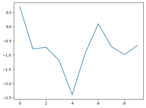
Below, the plt.plot function creates a chart (by default a line chart) and plt.show() "prints" it to the screen.
import matplotlib.pyplot as plt
import seaborn as sns
import pandas as pd
import numpy as np

df = pd.DataFrame({'random_numbers' : np.random.randn(10)})
print(df)

plt.plot(df)
plt.show()
   random_numbers
0        0.690745
1       -0.791721
2       -0.726929
3       -1.190095
4       -2.399059
5       -0.934381
6        0.099680
7       -0.708663
8       -0.983769
9       -0.661916
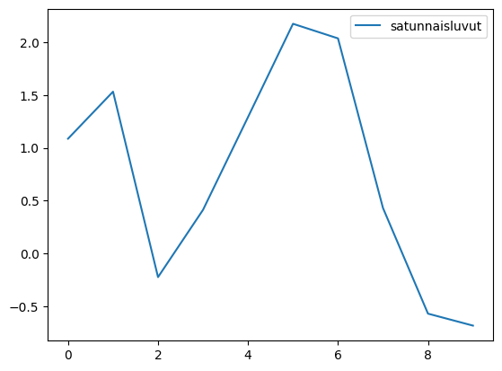
Here, an alternative syntax can also be used, where the plot method of the DataFrame is called. This also uses matplotlib.pyplot.
df = pd.DataFrame({'random_numbers' : np.random.randn(10)})
print(df)

df.plot()
plt.show()
   random_numbers
0        1.086314
1        1.531357
2       -0.223992
3        0.412642
4        1.290829
5        2.173870
6        2.035647
7        0.430138
8       -0.569746
9       -0.683068
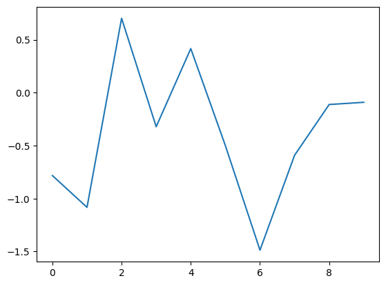
A third syntax is also in use:
df = pd.DataFrame({'random_numbers' : np.random.randn(10)})
print(df)

plt.plot('random_numbers', data=df)  # DataFrame used with the data parameter
plt.show()
   random_numbers
0       -0.783194
1       -1.082977
2        0.702581
3       -0.321643
4        0.415943
5       -0.500592
6       -1.487482
7       -0.591301
8       -0.112004
9       -0.091061
Often in Jupyter, plots are set to display automatically without the need for a plt.show() call. This can be achieved by running the command
%matplotlib inline
once in the Notebook, after which the chart will print with just the plot command.
Another way is to run the command
%matplotlib notebook
which gives an interactive view to Jupyter's charts.
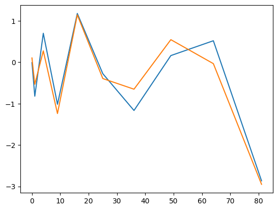
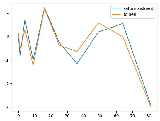
plt.plot thus draws a line chart. If a DataFrame is given as a parameter, its index becomes the horizontal axis, and each (numeric) column is drawn as its own series of values.
df = pd.DataFrame({'random_numbers' : np.random.randn(10)})
df['second'] = df['random_numbers'] + np.random.randn(10)/3
df.set_index(np.arange(0,10)**2, inplace = True)
print(df)

plt.plot(df)
plt.show()

# method2

df.plot()
plt.show()
    random_numbers    second
0        -0.011381  0.102051
1        -0.821388 -0.534439
4         0.697204  0.273066
9        -1.016818 -1.240141
16        1.175636  1.141187
25       -0.278707 -0.395595
36       -1.166327 -0.652345
49        0.158880  0.543259
64        0.517002 -0.035546
81       -2.864796 -2.948615
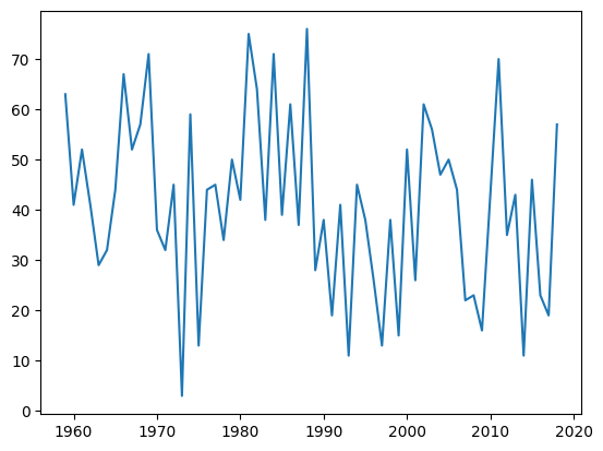
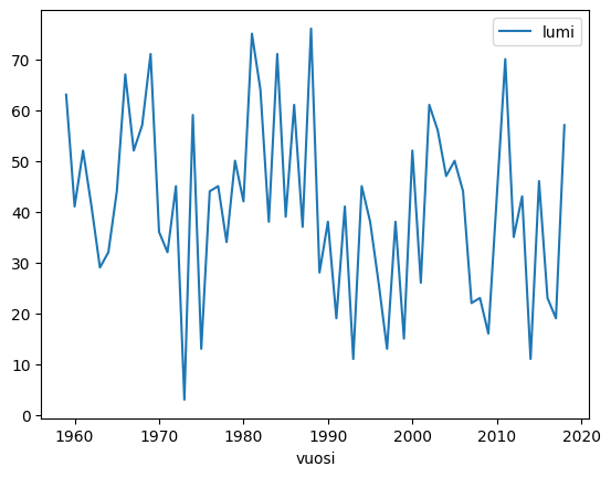
You can also specify the x and y axis values separately:
df = pd.read_csv('Datasets/snow.txt')
print(df.head())

plt.plot(df['year'], df['snow'])  # 1st parameter x, second y
plt.show()

# method2
df.plot('year', 'snow')  # 1st parameter x, second y
plt.show()
   year  snow
0   1959    63
1   1960    41
2   1961    52
3   1962    41
4   1963    29
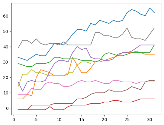
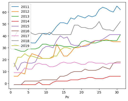
df = pd.read_csv('Datasets/years.txt')
print(df.head())

plt.plot(df['Dd'],df.iloc[:,1:]) # here Dd-column as x for all and other columns as y
plt.show()

# method2

df.plot('Dd',['2011','2012','2013','2014','2015','2016','2017','2018','2019']) # here Dd-column as x for all and other columns as y
plt.show()
   Dd  2011  2012  2013  2014  2015  2016  2017  2018  2019
0   1  33.0   6.0  29.0  -1.0  17.0  -1.0   9.0  39.0  14.0
1   2  32.0   6.0  28.0  -1.0  11.0  -1.0   9.0  44.0  22.0
2   3  31.0   9.0  27.0  -1.0  17.0  -1.0   9.0  44.0  22.0
3   4  33.0   8.0  27.0  -1.0  18.0   2.0  13.0  42.0  25.0
4   5  35.0  20.0  29.0  -1.0  17.0   2.0  12.0  45.0  23.0
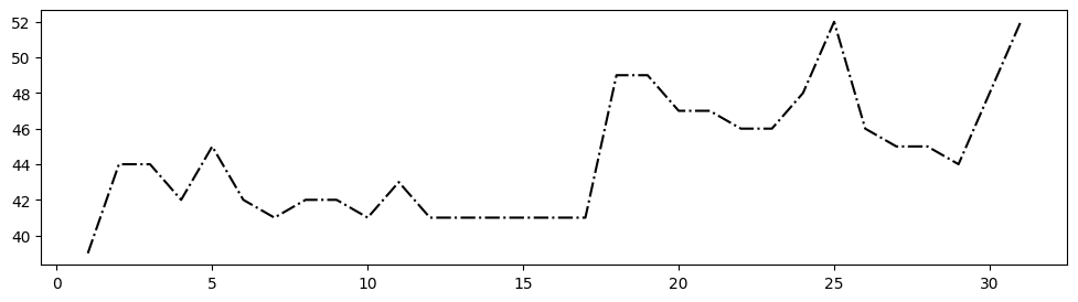
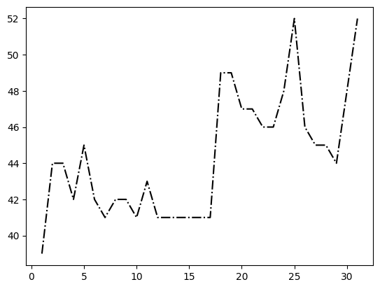
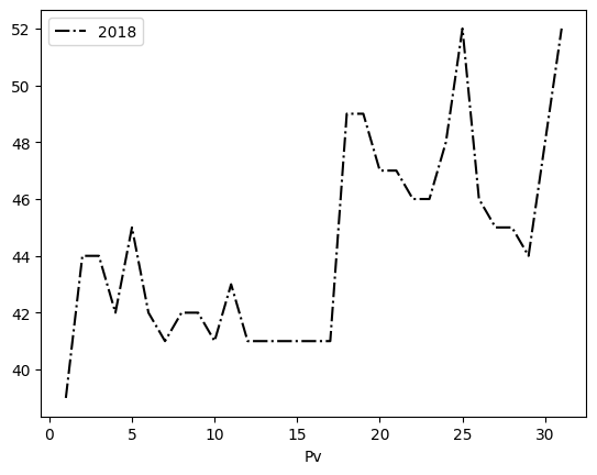
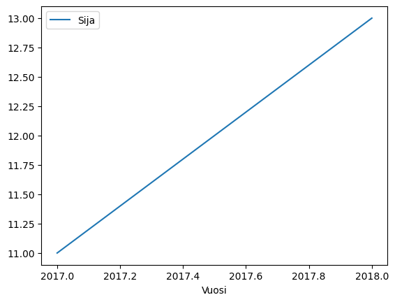
As the third parameter, you can give a formatting command, which is in the short form [color][marker][line]. For example, 'k-.' means a black dash-dot line:
df = pd.read_csv('Datasets/vuodet.txt')
print(df.head())

plt.plot(df['Pv'],df['2018'], 'k-.')
plt.show()

#method2

df.plot('Pv','2018', style='k-.')
plt.show()
   Pv  2011  2012  2013  2014  2015  2016  2017  2018  2019
0   1  33.0   6.0  29.0  -1.0  17.0  -1.0   9.0  39.0  14.0
1   2  32.0   6.0  28.0  -1.0  11.0  -1.0   9.0  44.0  22.0
2   3  31.0   9.0  27.0  -1.0  17.0  -1.0   9.0  44.0  22.0
3   4  33.0   8.0  27.0  -1.0  18.0   2.0  13.0  42.0  25.0
4   5  35.0  20.0  29.0  -1.0  17.0   2.0  12.0  45.0  23.0
The specifications for the formatting commands can be found in the Notes section of the API.
If there are multiple series of values and different formats are desired for them, the parameters are given in method 1 as x,y,format triplets, and in method 2 as a list in the style parameter.
Often the axis titles are important explanatory factors, they can be added with the methods xlabel, ylabel. The overall chart title is added with the method title and the legend can be displayed with the method legend. In method 2, the legend comes automatically.
df = pd.read_csv('Datasets/vuodet.txt')
print(df.head())
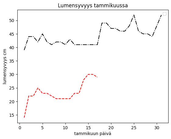
plt.plot(df['Pv'],df['2018'], 'k-.', df['Pv'],df['2019'], 'r--') # here the Pv column is used for all x's and other columns for y's
plt.xlabel('January day')
plt.ylabel('snow depth cm')
plt.title('Snow depth in January')
plt.legend()
plt.show()
# method2, legend comes automatically
df.plot('Pv',['2018', '2019'], style=['k-.','r--'])
plt.ylabel('snow depth cm')
plt.title('Snow depth in January')
plt.show()
No artists with labels found to put in legend. Note that artists whose label start with an underscore are ignored when legend() is called with no argument.
Day 2011 2012 2013 2014 2015 2016 2017 2018 2019 0 1 33.0 6.0 29.0 -1.0 17.0 -1.0 9.0 39.0 14.0 1 2 32.0 6.0 28.0 -1.0 11.0 -1.0 9.0 44.0 22.0 2 3 31.0 9.0 27.0 -1.0 17.0 -1.0 9.0 44.0 22.0 3 4 33.0 8.0 27.0 -1.0 18.0 2.0 13.0 42.0 25.0 4 5 35.0 20.0 29.0 -1.0 17.0 2.0 12.0 45.0 23.0
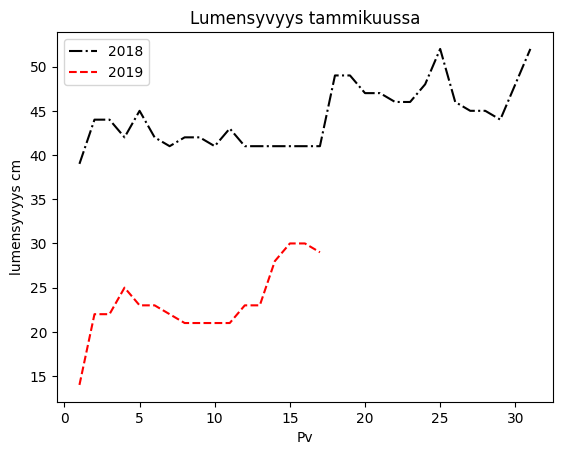
Here we saw that in method 1, the legend incorrectly places the title for the second line (2018), meaning matplotlib failed in automatic determination. The titles for the legend can be listed in the legend method.
df = pd.read_csv('Datasets/years.txt')
print(df.head())

plt.plot(df['Day'],df['2018'], 'k-.', df['Day'],df['2019'], 'r--') # here Day column as x for all and other columns as y
plt.xlabel('day of January')
plt.ylabel('snow depth cm')
plt.title('Snow depth in January')
plt.legend([2018,2019])
plt.show()
   Day  2011  2012  2013  2014  2015  2016  2017  2018  2019
0   1  33.0   6.0  29.0  -1.0  17.0  -1.0   9.0  39.0  14.0
1   2  32.0   6.0  28.0  -1.0  11.0  -1.0   9.0  44.0  22.0
2   3  31.0   9.0  27.0  -1.0  17.0  -1.0   9.0  44.0  22.0
3   4  33.0   8.0  27.0  -1.0  18.0   2.0  13.0  42.0  25.0
4   5  35.0  20.0  29.0  -1.0  17.0   2.0  12.0  45.0  23.0
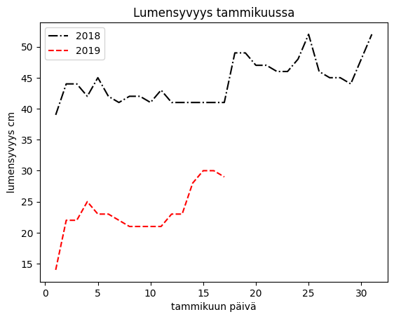
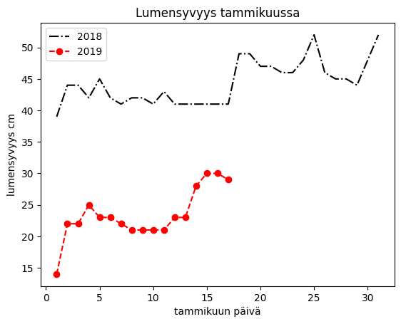
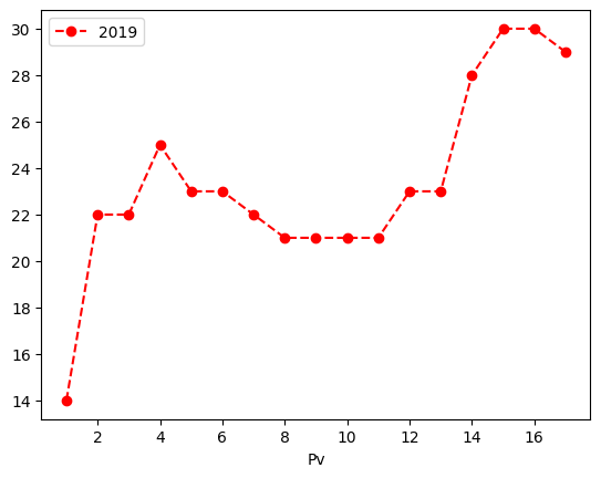
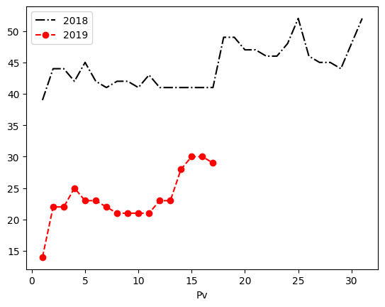
New data series can also be added to an already created chart and the title can be defined at the same time with the label parameter:
df = pd.read_csv('Datasets/years.txt')
print(df.head())

plt.plot(df['Day'],df['2018'], 'k-.', label=2018)
plt.plot(df['Day'],df['2019'], 'ro--', label=2019)  # ro-- adds round markers
plt.xlabel('January day') plt.ylabel('Snow depth in cm') plt.title('Snow Depth in January') plt.legend() plt.show()
   Day  2011  2012  2013  2014  2015  2016  2017  2018  2019
0   1  33.0   6.0  29.0  -1.0  17.0  -1.0   9.0  39.0  14.0
1   2  32.0   6.0  28.0  -1.0  11.0  -1.0   9.0  44.0  22.0
2   3  31.0   9.0  27.0  -1.0  17.0  -1.0   9.0  44.0  22.0
3   4  33.0   8.0  27.0  -1.0  18.0   2.0  13.0  42.0  25.0
4   5  35.0  20.0  29.0  -1.0  17.0   2.0  12.0  45.0  23.0
In the second way, these will appear in different charts:
```python
df = pd.read_csv('Datasets/years.txt')
print(df.head())
# method2
df.plot('Day','2018', style='k-.')
df.plot('Day','2019', style='ro--') # ro-- adds round markers
plt.show()
Day 2011 2012 2013 2014 2015 2016 2017 2018 2019
0 1 33.0 6.0 29.0 -1.0 17.0 -1.0 9.0 39.0 14.0
1 2 32.0 6.0 28.0 -1.0 11.0 -1.0 9.0 44.0 22.0
2 3 31.0 9.0 27.0 -1.0 17.0 -1.0 9.0 44.0 22.0
3 4 33.0 8.0 27.0 -1.0 18.0 2.0 13.0 42.0 25.0
4 5 35.0 20.0 29.0 -1.0 17.0 2.0 12.0 45.0 23.0

To get them into the same chart, you can capture the Axes-type object returned by df.plot and pass it as the ax parameter to the second df.plot. More on the Axes object below.
df = pd.read_csv('Datasets/years.txt')
print(df.head())

# method2

ax1 = df.plot('Day','2018', style='k-.')
df.plot('Day','2019', style='ro--', ax=ax1)  # ro-- adds round markers
plt.show()
Year 2011 2012 2013 2014 2015 2016 2017 2018 2019 0 1 33.0 6.0 29.0 -1.0 17.0 -1.0 9.0 39.0 14.0 1 2 32.0 6.0 28.0 -1.0 11.0 -1.0 9.0 44.0 22.0 2 3 31.0 9.0 27.0 -1.0 17.0 -1.0 9.0 44.0 22.0 3 4 33.0 8.0 27.0 -1.0 18.0 2.0 13.0 42.0 25.0 4 5 35.0 20.0 29.0 -1.0 17.0 2.0 12.0 45.0 23.0
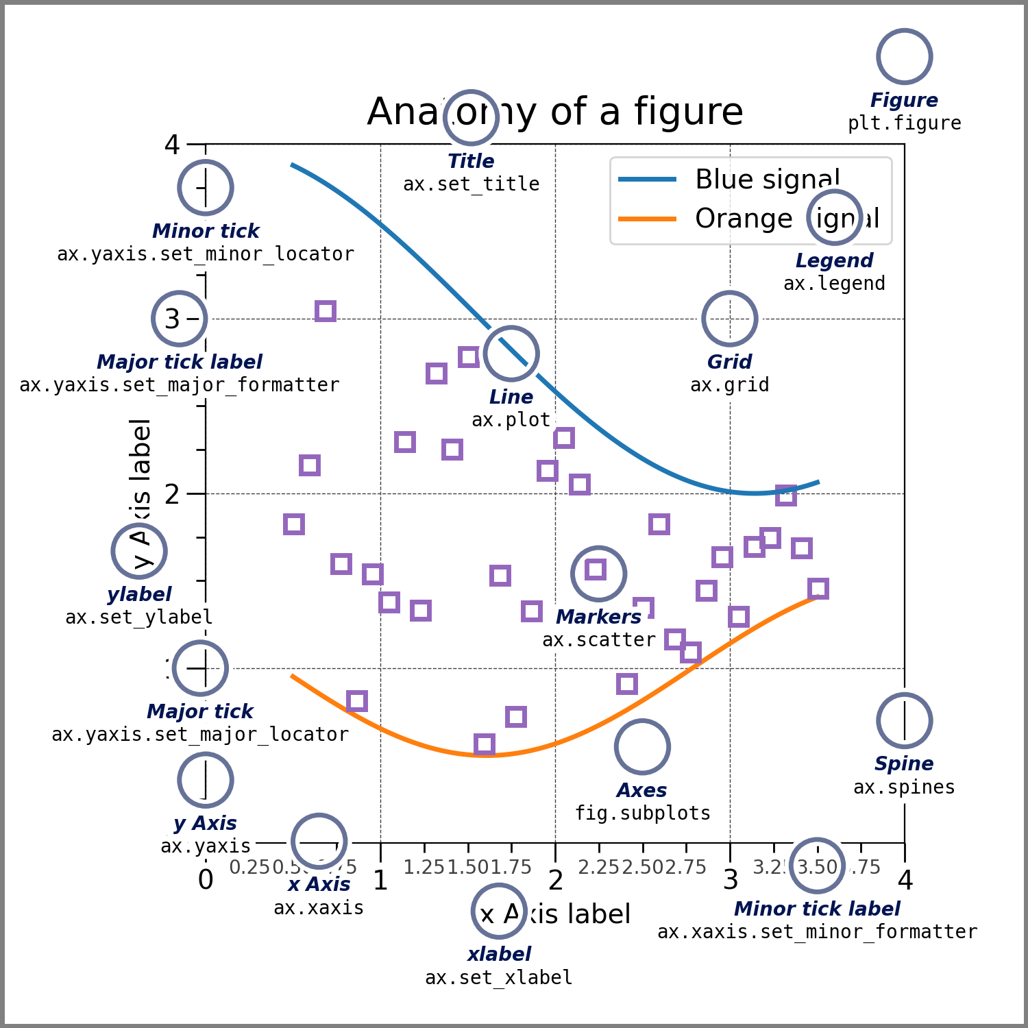
Different parts of the chart can be formatted almost endlessly:
Multiple Charts
The concept of pyplot is based on the idea of the current figure and current chart: all plt. methods are done on the current chart, which is located in the current figure.
figurea figure, which can contain multiple chartsaxesa chart (which is always located in some figure). Does not mean axis (=axis)
If only one chart is drawn, there is no need to worry about these, as figures and their charts are created "under the hood".
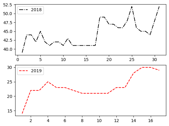
But it is also possible to draw several charts in the same figure:
df = pd.read_csv('Datasets/years.txt')
print(df.head())

plt.figure()  # create a new figure, this is the "current figure". Unnecessary, because the figure also always comes automatically
plt.subplot(2,1,1)  # make a 2 row, 1 column "grid" in the current figure and take the 1st place as the "current chart"
plt.plot(df['Year'],df['2018'], 'k-.', label=2018) # draw on the "current chart"
plt.legend() # add a legend to the "current chart"
plt.subplot(2,1,2) # take the 2nd place of the "current figure" as the "current chart"
plt.plot(df['Year'],df['2019'], 'r--', label=2019)# draw on the "current chart"
plt.legend() # add a legend to the "current chart"
plt.show() # display the current figure
Year 2011 2012 2013 2014 2015 2016 2017 2018 2019 0 1 33.0 6.0 29.0 -1.0 17.0 -1.0 9.0 39.0 14.0 1 2 32.0 6.0 28.0 -1.0 11.0 -1.0 9.0 44.0 22.0 2 3 31.0 9.0 27.0 -1.0 17.0 -1.0 9.0 44.0 22.0 3 4 33.0 8.0 27.0 -1.0 18.0 2.0 13.0 42.0 25.0 4 5 35.0 20.0 29.0 -1.0 17.0 2.0 12.0 45.0 23.0
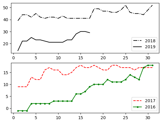
In the plt.subplot(2,1,1) annotation, you can also use a single parameter 211 if the numbers are <10
df = pd.read_csv('Datasets/years.txt')
print(df.head())

plt.figure()  # create a new figure, this is the "current figure". Unnecessary, because the figure always comes automatically as well
plt.subplot(211)  # make a 2 row, 1 column "grid" in the current figure and take the 1st place as the "current chart"
plt.plot(df['Year'],df['2018'], 'k-.', label=2018) # draw on the "current chart"
plt.legend() # add a legend to the "current chart"
plt.subplot(212) # take the 2nd place of the "current figure" as the "current chart"
plt.plot(df['Year'],df['2017'], 'r--', label=2017)# draw on the "current chart"
plt.plot(df['Year'],df['2016'], 'g.-', label=2016)# draw on the "current chart"
plt.legend() # add a legend to the "current chart"

plt.subplot(211)  # switch back to the 1st chart
plt.plot(df['Year'],df['2019'], 'k-', label=2019) # draw on the "current chart"
plt.legend()
plt.show() # display the current figure
Pv 2011 2012 2013 2014 2015 2016 2017 2018 2019 0 1 33.0 6.0 29.0 -1.0 17.0 -1.0 9.0 39.0 14.0 1 2 32.0 6.0 28.0 -1.0 11.0 -1.0 9.0 44.0 22.0 2 3 31.0 9.0 27.0 -1.0 17.0 -1.0 9.0 44.0 22.0 3 4 33.0 8.0 27.0 -1.0 18.0 2.0 13.0 42.0 25.0 4 5 35.0 20.0 29.0 -1.0 17.0 2.0 12.0 45.0 23.0
If multiple figures are desired, a number is given to the plt.figure function to return to the figure:
df = pd.read_csv('Datasets/years.txt')
print(df.head())

plt.figure(1)
plt.plot(df['Pv'],df['2018'], 'k-.', label=2018)
plt.legend()

plt.figure(2)
plt.plot(df['Pv'],df['2016'], 'g.-', label=2016)
plt.legend()

plt.figure(1)
plt.plot(df['Pv'],df['2019'], 'k-', label=2019)
plt.legend()

plt.show()
   Pv  2011  2012  2013  2014  2015  2016  2017  2018  2019
0   1  33.0   6.0  29.0  -1.0  17.0  -1.0   9.0  39.0  14.0
1   2  32.0   6.0  28.0  -1.0  11.0  -1.0   9.0  44.0  22.0
2   3  31.0   9.0  27.0  -1.0  17.0  -1.0   9.0  44.0  22.0
3   4  33.0   8.0  27.0  -1.0  18.0   2.0  13.0  42.0  25.0
4   5  35.0  20.0  29.0  -1.0  17.0   2.0  12.0  45.0  23.0

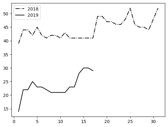
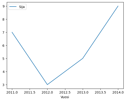
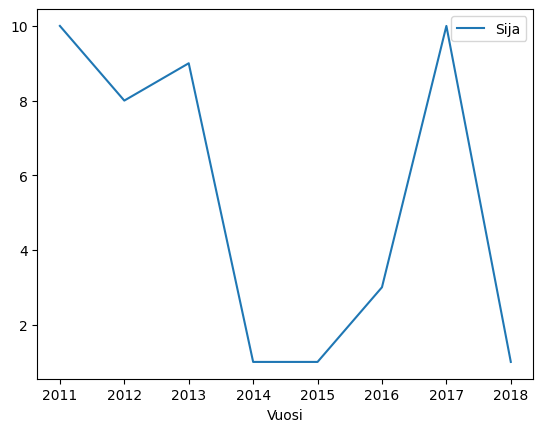
Chart from Groupby
The plot method can also be called on a GroupBy object, by default this results in a separate chart for each group.
df = pd.read_csv('Datasets/league.txt')
print(df)

df.groupby('Team').plot('Year', 'Rank')
plt.show()
Year Team Rank 0 2011 JYP 4 1 2012 JYP 1 2 2013 JYP 3 3 2014 JYP 5 4 2015 JYP 3 5 2016 JYP 4 6 2017 JYP 3 7 2018 JYP 5 8 2017 Jukurit 11 9 2018 Jukurit 13 10 2011 Jokerit 7 11 2012 Jokerit 3 12 2013 Jokerit 5 13 2014 Jokerit 9 14 2011 Kärpät 10 15 2012 Kärpät 8 16 2013 Kärpät 9 17 2014 Kärpät 1 18 2015 Kärpät 1 19 2016 Kärpät 3 20 2017 Kärpät 10 21 2018 Kärpät 1
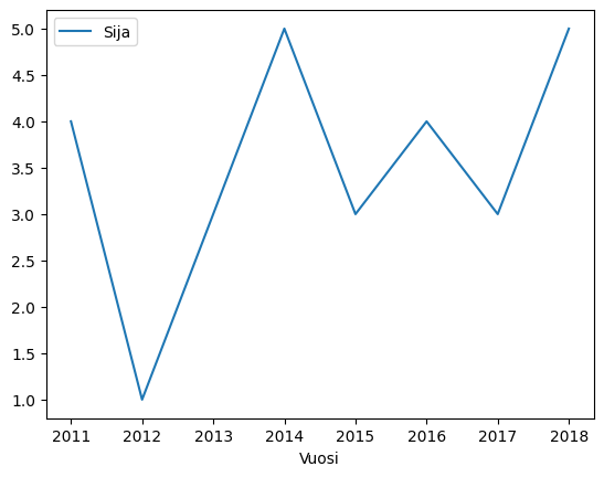
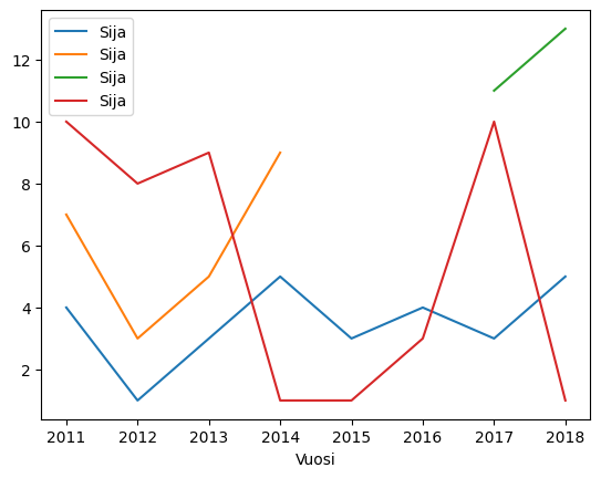
The same chart can be obtained by saving the "current figure" object given by plt into a variable and passing it as the ax parameter to plot:
df = pd.read_csv('Datasets/liiga.txt')

fig1, ax1 = plt.subplots()

df.groupby('Team').plot('Year', 'Rank', ax=ax1)
plt.show()
Other types of charts
plot thus makes a line chart, other types of charts can be obtained with functions such as
* bar for bar chart
* barh for horizontal bar chart
* pie for pie chart
* scatter for scatter plot, where the size and color of the points can vary
* hist for histogram, i.e., distribution by category
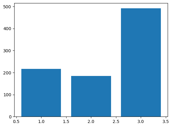
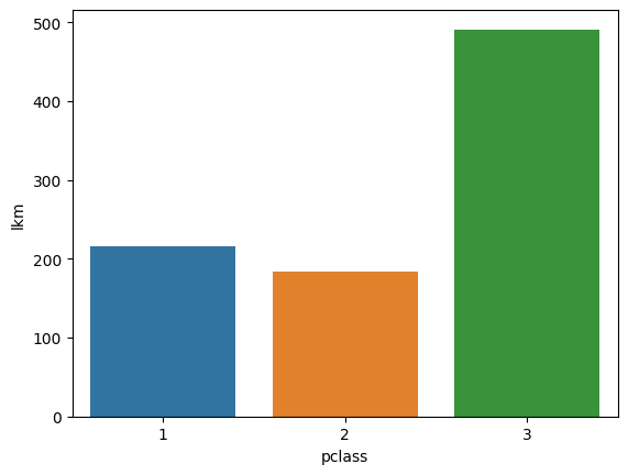
Let's return to the Titanic data and calculate some summaries:
df = pd.read_csv('Datasets/titanic.csv', index_col=0)
df2 = df['Pclass'].value_counts(sort=False)
print(df2)
plt.bar(df2.index, df2) #or df2.plot.bar(), which is often easier if the DataFrame's index has "sensible values"
plt.show()
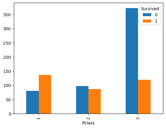
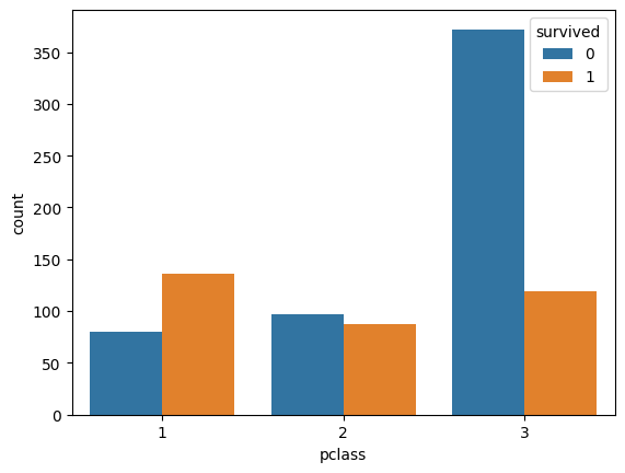
df3 = pd.crosstab(df['Pclass'], df['Survived'])
print(df3)
df3.plot.bar()
plt.show()
# another way to achieve the same
df3.plot(kind='bar')
plt.show()
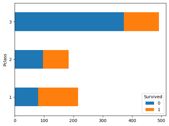
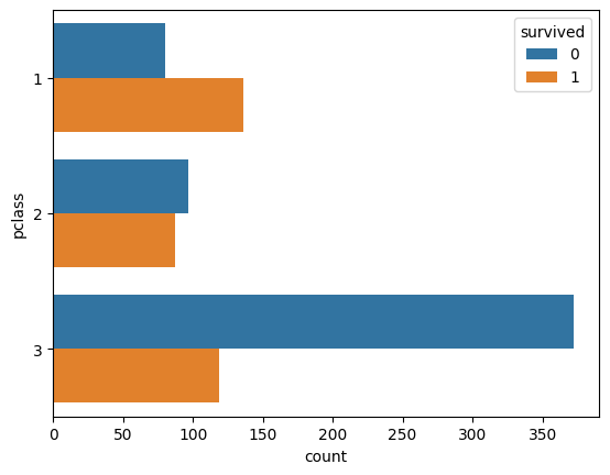
df3.plot.barh(stacked = True)
plt.show()
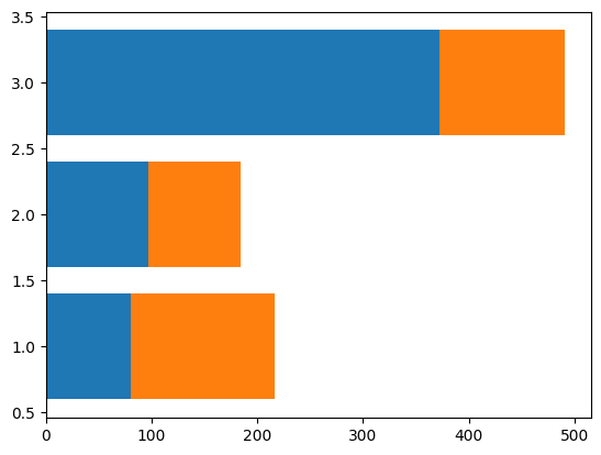
# way2
plt.barh(df3.index, df3[0]) # class-axis values, heights of the bars (here "lengths")
plt.barh(df3.index, df3[1], left = df3[0]) # left indicates where the bars start, this way we get a stacked chart
plt.show()
3    491
1    216
2    184
Name: Pclass, dtype: int64
Survived 0 1
Pclass
1 80 136
2 97 87
3 372 119

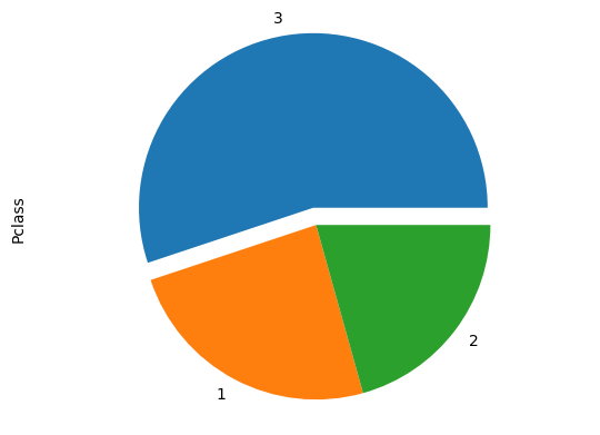
Example of a pie chart:
```python
df4 = df['Pclass'].value_counts(sort=False)
df4.plot.pie(explode = [0.1,0,0])
plt.axis('equal') # this makes a circle, otherwise it would be an ellipse
plt.show()
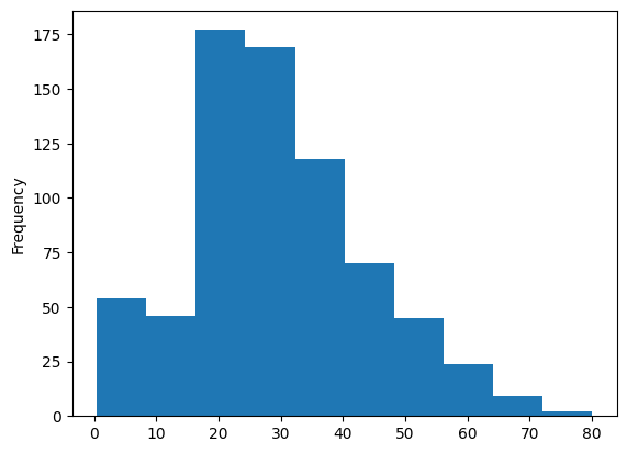
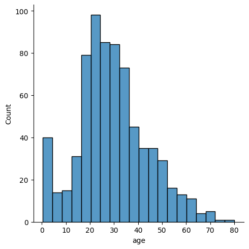
Histogram
A histogram can be made directly from the original dataset. The values belonging to different classes do not need to be counted separately in the DataFrame.
Density turns it into a "continuous distribution".
df = pd.read_csv('Datasets/titanic.csv', index_col=0)

df['Age'].plot.hist()  # here the classes are defined automatically
plt.show()
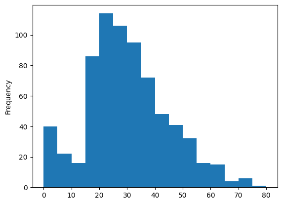
df['Age'].plot.hist(bins=np.arange(0,85,5)) # classes given as a list [0,5,10,...,80]
plt.show()
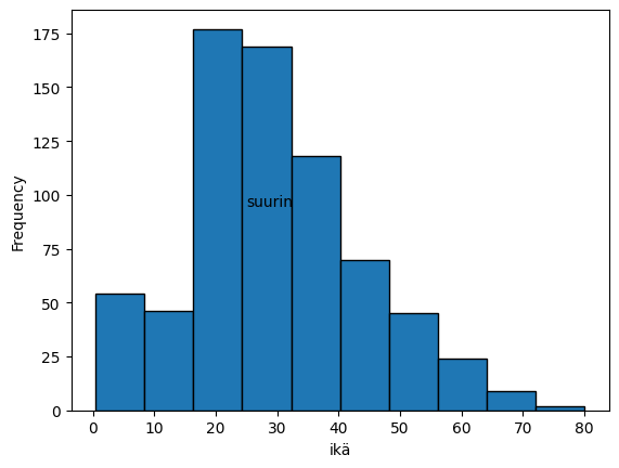
df['Age'].plot.hist(20, edgecolor='black') # number of classes, color of the bar edges
plt.xlabel('age')
plt.annotate('largest',(25,95))  # this adds text to the chart
plt.show()
Seaborn Library
Seaborn is a library built on top of the matplotlib library, offering an easy interface for creating many otherwise difficult-to-make charts.
This section mainly introduces the features of the Seaborn library. These will not be covered in detail in this course module.
The Seaborn library also contains a similar titanic dataset for practice:
# Titanic dataset is available in Seaborn by default
titanic = sns.load_dataset('titanic')
titanic.head()
| survived | pclass | sex | age | sibsp | parch | fare | embarked | class | who | adult_male | deck | embark_town | alive | alone | |
|---|---|---|---|---|---|---|---|---|---|---|---|---|---|---|---|
| 0 | 0 | 3 | male | 22.0 | 1 | 0 | 7.2500 | S | Third | man | True | NaN | Southampton | no | False |
| 1 | 1 | 1 | female | 38.0 | 1 | 0 | 71.2833 | C | First | woman | False | C | Cherbourg | yes | False |
| 2 | 1 | 3 | female | 26.0 | 0 | 0 | 7.9250 | S | Third | woman | False | NaN | Southampton | yes | True |
| 3 | 1 | 1 | female | 35.0 | 1 | 0 | 53.1000 | S | First | woman | False | C | Southampton | yes | False |
| 4 | 0 | 3 | male | 35.0 | 0 | 0 | 8.0500 | S | Third | man | True | NaN | Southampton | no | True |
countplot
Seaborn's countplot provides an easy way to present counts:
titanic = sns.load_dataset('titanic')
sns.countplot(x='pclass', data=titanic)
plt.show()

# another way

sns.countplot(titanic['pclass'])
plt.show()

There is no need to count the quantities separately, as seaborn takes care of the computation.
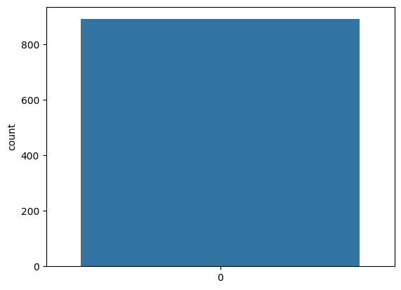
The chart can be modified after creation by saving the Axes object returned by countplot to a variable:
```python
ax = sns.countplot(x='pclass', data=titanic)
ax.set_ylabel('count') # also plt.ylabel('count') would work for modifying the current chart
plt.show()
The hue parameter can be used to include a second classification column:
ax = sns.countplot(x='pclass', hue='survived', data=titanic)
plt.show()
And horizontal bars can be created by providing y instead of x. In seaborn functions, the DataFrame to be used is usually given in the data parameter, and the names of the columns are given as x/y/hue etc. parameters.
ax = sns.countplot(y='pclass', hue='survived', data=titanic)
plt.show()
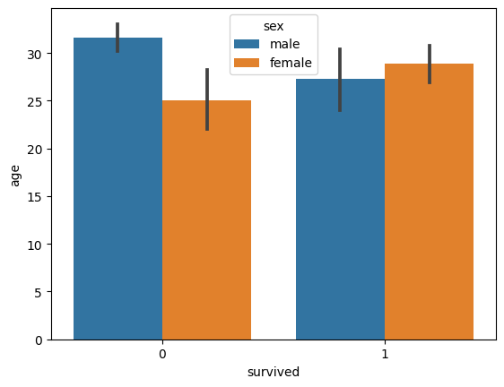
barplot
barplot creates a bar chart that by default shows the means and the confidence intervals of the means (at a 95% significance level).
sns.barplot(x='survived', y='age', hue='sex', data=titanic)
plt.show()
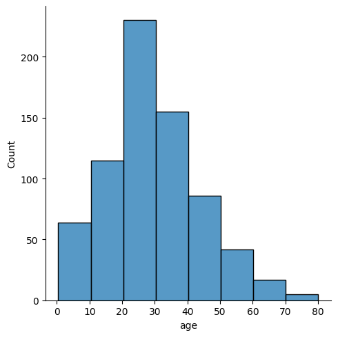
distplot
distplot creates an overlapping histogram and an estimated density function of the distribution. This function takes a Series directly as a parameter. NaN values cause an error here, so they are dropped with dropna().
sns.displot(titanic['age'].dropna())
plt.show()
sns.displot(titanic['age'].dropna(), kde=False, bins=8) # kde=False creates only the histogram, hist=False would create only the density function
plt.show()
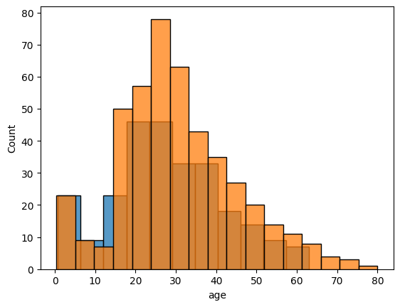
Two distributions can be plotted in the same chart by saving the Axes object and passing it as the ax parameter:
ax1 = sns.histplot(titanic[titanic['sex']=='female']['age'].dropna(), kde=False)
sns.histplot(titanic[titanic['sex']=='male']['age'].dropna(), kde=False, ax=ax1)
plt.show()
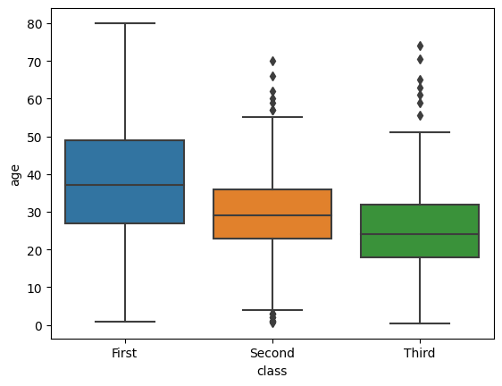
boxplot
boxplot creates a so-called box-and-whisker plot, which can easily depict the distribution of numerical values by category. The boxes contain 50% of the values from the center of the distribution, and the whiskers extend to 1.5 times the height of the box above and below. Values outside these are plotted as outliers.
sns.boxplot(x='class', y='age', data=titanic)
plt.show()
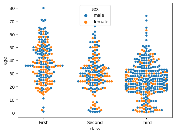
swarmplot
swarmplot depicts individual values by category.
sns.swarmplot(x='class', y='age', hue='sex', data=titanic)
plt.show()
C:\Users\mikar\Anaconda3\envs\Threat-DA\lib\site-packages\seaborn\categorical.py:3540: UserWarning: 15.2% of the points cannot be placed; you may want to decrease the size of the markers or use stripplot.
  warnings.warn(msg, UserWarning)
C:\Users\mikar\Anaconda3\envs\Threat-DA\lib\site-packages\seaborn\categorical.py:3540: UserWarning: 15.2% of the points cannot be placed; you may want to decrease the size of the markers or use stripplot.
  warnings.warn(msg, UserWarning)
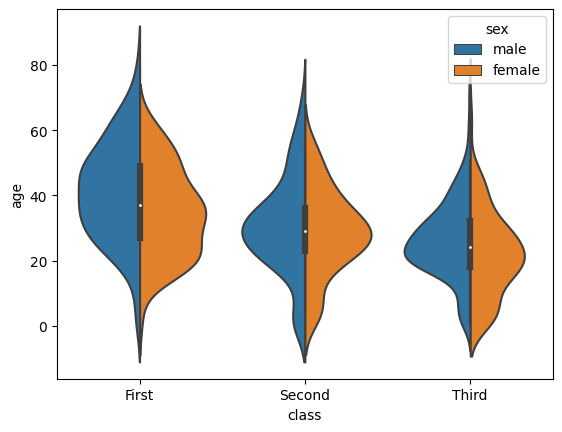
violinplot
violinplot displays the same distributions as continuous distributions.
sns.violinplot(x='class', y='age', hue='sex', split=True, data=titanic)
plt.show()
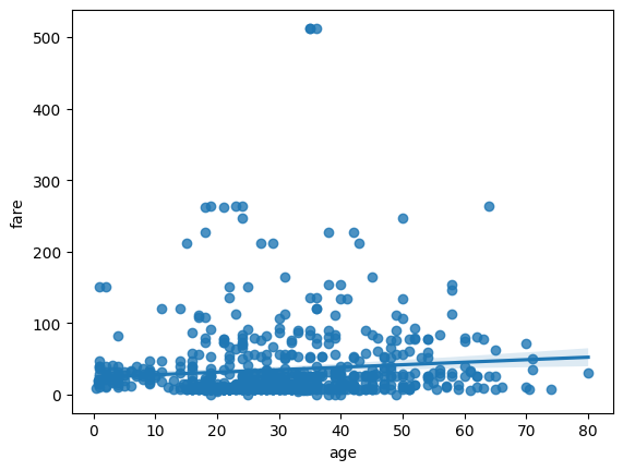
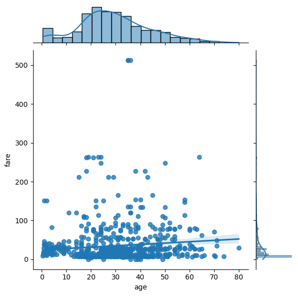
regplot, jointplot
regplot defines a regression line between two variables. jointplot adds histograms for both to this.
sns.regplot(data=titanic, x='age', y='fare')
plt.show()
sns.jointplot(data=titanic, x='age', y='fare', kind='reg')
plt.show()
pairplot
pairplot draws distributions from several variable pairs at the same time.
sns.pairplot(titanic[['age', 'fare', 'sibsp', 'survived']].dropna(), kind='reg')
plt.show()

sns.pairplot(titanic[['age', 'fare', 'sibsp', 'survived', 'sex']].dropna(), kind='reg', hue='sex')
plt.show()
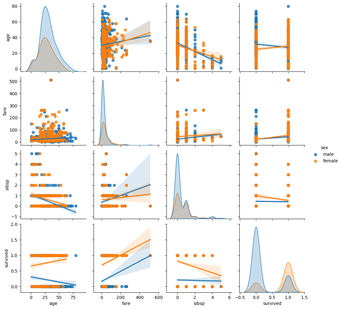
Figure size and saving
The figure size can be defined in inches, the default size is 6.4 x 4.8 inches.
df = pd.read_csv('Datasets/years.txt')

plt.plot(df['Day'],df['2018'], 'k-.')

fig = plt.gcf()  #gives the current figure
fig.set_size_inches(12, 3)

plt.show()

The figure can be saved with the savefig function. If the format parameter is not given, the file format is inferred from the file extension. Most environments support at least the formats png, pdf, ps, eps, and svg.
df = pd.read_csv('Datasets/years.txt')

plt.plot(df['Day'],df['2018'], 'k-.')

fig = plt.gcf()  #gives the current figure
fig.set_size_inches(12, 3)
plt.savefig('figure1.png', dpi=400)
plt.show()